PrmsDiscretization and PrmsPlot

In this tutorial we give a quick rundown of how to import a discretization for a PRMS model and how to plot figures using it’s discretization.

This tutorial presents two methods to create a PrmsDiscretization object: - from a FloPy model object - from a shapefile

This tutorial then shows how to use the PrmsDiscretization object with PrmsPlot to create figures

import os
from gsflow import GsflowModel
from gsflow.output import PrmsDiscretization, PrmsPlot
import matplotlib.pyplot as plt
import numpy as np
import os

To start this tutorial, let’s load the Sagehen model to work with

workspace = os.path.join(".", "data", "sagehen", "gsflow")
control = "saghen_new_cont.control"

gsf = GsflowModel.load_from_file(os.path.join(workspace, control))

Control file is loaded
Working on loading PRMS model ...
Prms model loading ...
------------------------------------
Reading parameter file : saghen_new_par_0.params
------------------------------------
Warning: ncascade data type will be infered from data supplied
Warning: ncascdgw data type will be infered from data supplied
Warning: ndays data type will be infered from data supplied
Warning: ndepl data type will be infered from data supplied
Warning: ndeplval data type will be infered from data supplied
Warning: nevap data type will be infered from data supplied
Warning: ngw data type will be infered from data supplied
Warning: ngwcell data type will be infered from data supplied
Warning: nhru data type will be infered from data supplied
Warning: nhrucell data type will be infered from data supplied
Warning: nlake data type will be infered from data supplied
Warning: nlake_hrus data type will be infered from data supplied
Warning: nmonths data type will be infered from data supplied
Warning: nobs data type will be infered from data supplied
Warning: nrain data type will be infered from data supplied
Warning: nreach data type will be infered from data supplied
Warning: nsegment data type will be infered from data supplied
Warning: nsnow data type will be infered from data supplied
Warning: nsol data type will be infered from data supplied
Warning: nssr data type will be infered from data supplied
Warning: nsub data type will be infered from data supplied
Warning: ntemp data type will be infered from data supplied
Warning: one data type will be infered from data supplied
------------------------------------
Reading parameter file : saghen_new_par_1.params
------------------------------------
------------------------------------
Reading parameter file : saghen_new_par_2.params
------------------------------------
------------------------------------
Reading parameter file : saghen_new_par_3.params
------------------------------------
PRMS model loaded ...
Working on loading MODFLOW files ....
   loading iuzfbnd array...
   loading irunbnd array...
   loading vks array...
   loading eps array...
   loading thts array...
stress period 1:
   loading finf array...
stress period 2:
MODFLOW files are loaded ...

Loading discretization from flopy

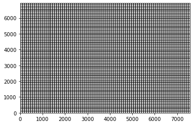
We can load our discretization from the Modflow model object if the hru’s in PRMS are consistent with modflow grid cells. The PrmsDiscretization object internally loads discretization information from the Modflow.modelgrid object

We can also plot the discretization from the PrmsDiscretization object

mf = gsf.mf
prms_dis = PrmsDiscretization.load_from_flopy(mf)
prms_dis.plot_discretization();

Load discretization from a shapefile

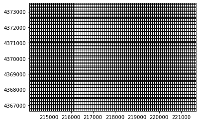
We can also load the hru discretization from a shapefile. PRMS HRU shapes and sizes do not have to correspond to the modflow grid and in this case, loading from a shapefile is necessary for plotting.

workspace = os.path.join(".", "data", "sagehen", "shapefiles")
shp = "hru_params.shp"

prms_dis = PrmsDiscretization.load_from_shapefile(os.path.join(workspace, shp))
prms_dis.plot_discretization();

Using PrmsPlot with the PrmsDiscretization object

PrmsPlot can be instatiated easily by passing it a PrmsDiscetizaiton object

We can use this to plot parameters from the parameter file, contour parameters, plot arrays of data, and contour arrays of data

# remember, prms_dis was loaded from our shapefile
plot = PrmsPlot(prms_dis)
PrmsPlot

gsflow.output.prms_plot.PrmsPlot

Plotting parameters

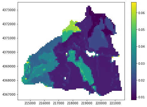
the plotting functions use matplotlib and accept matplotlib keyword arguments. In addition a masked_value argument can be supplied to mask out certain values

plot = PrmsPlot(prms_dis)

fig = plt.figure(figsize=(8, 6))

# let's grab a parameter to plot
ssr2gw = gsf.prms.parameters.get_record("ssr2gw_rate")

# mask out 0 value and set the colormap to viridis
ax = plot.plot_parameter(ssr2gw, masked_values=[0], cmap="viridis")
plt.colorbar(ax);

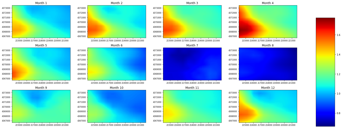
If a parameter has a dimension of nhru*12 we can plot that too:

let’s use rain_adj as an example, we automatically add the colorbar for these parameters so there is no need for the user to

rain_adj = gsf.prms.parameters.get_record("rain_adj")

# mask out 0 value and set the colormap to jet
ax = plot.plot_parameter(rain_adj, masked_values=[0], cmap="jet")

Contouring a parameter

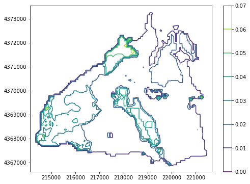
contouring a parameter is very easy using the contour_parameter() method. This method also accepts matplotlib keyword arguments for contouring and has a masked_values argument

plot = PrmsPlot(prms_dis)

fig = plt.figure(figsize=(8, 6))

# let's grab a parameter to plot
ssr2gw = gsf.prms.parameters.get_record("ssr2gw_rate")

# set the colormap to viridis
ax = plot.contour_parameter(ssr2gw, cmap="viridis")
plt.colorbar(ax);

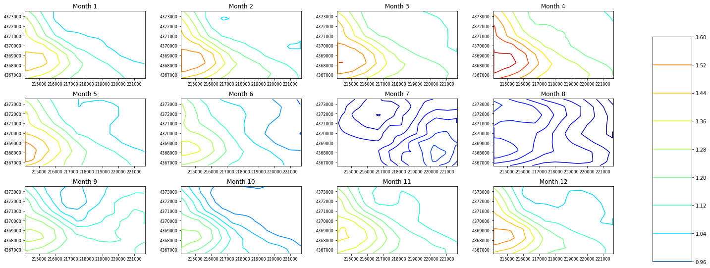
If a parameter has a dimension of nhru*12 we can contour that too:

let’s use rain_adj as an example, we automatically add a scale for these parameters so there is no need for the user to

rain_adj = gsf.prms.parameters.get_record("rain_adj")

# mask out 0 value and set the colormap to jet
ax = plot.contour_parameter(rain_adj, masked_values=[0], cmap="jet")

Plotting and Contouring external data

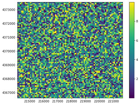
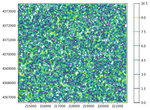
PrmsPlot supports plotting and contouring external data with the plot_array and contour_array method.

Of note: the array of data must be the same size as nhru

array = np.random.rand(prms_dis.nhru) * 10

fig = plt.figure(figsize=(8, 6))
plot = PrmsPlot(prms_dis)
ax = plot.plot_array(array)
plt.colorbar(ax);

fig = plt.figure(figsize=(8, 6))
ax = plot.contour_array(array)
plt.colorbar(ax);

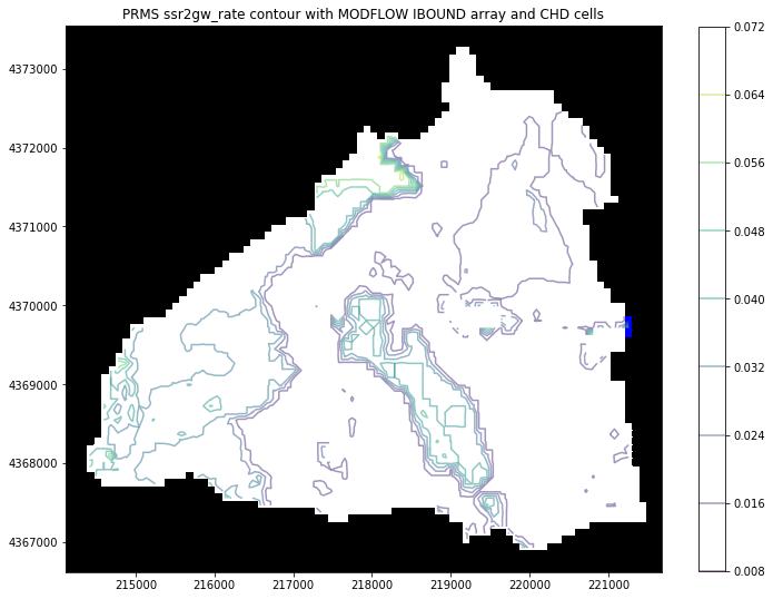
The PrmsPlot class is compatible with flopy

Plotting using PrmsPlot can be layered with flopy’s PlotMapView to create gsflow plots!

Let’s look at a basic example

import flopy as fp
from flopy.plot import PlotMapView

fig = plt.figure(figsize=(12, 12))


# get the gsflow modflow object and pass it to flopy's ModelMap
ml = gsf.mf
ml.modelgrid.set_coord_info(xoff=prms_dis.extent[0], yoff=prms_dis.extent[2])
m_map = PlotMapView(model=ml)
m_map.plot_ibound()
# get the current working matplotlib axes object
flopy_ax = plt.gca()

# let's grab a prms parameter to plot
ssr2gw = gsf.prms.parameters.get_record("ssr2gw_rate")
plot = PrmsPlot(prms_dis)
# let's pass the flopy_ax to contour_parameter()
ax = plot.contour_parameter(ssr2gw, ax=flopy_ax, masked_values=[0], cmap="viridis", alpha=0.5)
plt.title("PRMS ssr2gw_rate contour with MODFLOW IBOUND array and CHD cells")
plt.colorbar(ax, shrink=0.75);