Creating a stream vector shapefile
pyGSFLOW includes capabilities for converting a discretized SFR stream network to a vector based shapefile. The attribute tabble of this shapefile contains information on each vector’s connectivity and can be used to parameterize MODSIM models.
The Modsim class in pyGSFLOW calculates stream segment connectivity to other segments and to lakes parameterized in the LAK package.
[1]:
# start with importing our packages
import os
import sys
import flopy as fp
import gsflow
import matplotlib.pyplot as plt
import numpy as np
import shapefile
import pandas as pd
[2]:
# define our model workspace and spatial information
ws = os.path.abspath(os.path.dirname(sys.argv[0]))
model_ws = os.path.join("data", "sagehen", "gsflow")

xll = 438979.0
yll = 3793007.75
angrot = 4
Loading a GSFLOW model
Our first step is to load a GSFLOW model using pyGSFLOW. If the model_mode parameter is set to MODSIM-GSFLOW or GSFLOW-MODSIM within the control file, pyGSFLOW will automatically create a stream vector shapefile when the model is written to disk. If the model_mode parameter in the GSFLOW control file is GSFLOW or MODFLOW the user can still create a stream vector shapefile. This example outlines how to create a shapefile in the second case (model_mode= GSFLOW or
MODFLOW)
[3]:
# load the model
gsf = gsflow.GsflowModel.load_from_file(os.path.join(model_ws, 'saghen_new_cont.control'))

# set model grid coordinate info
gsf.mf.modelgrid.set_coord_info(xll, yll, 4)
Control file is loaded
Working on loading PRMS model ...
Prms model loading ...
------------------------------------
Reading parameter file : saghen_new_par_0.params
------------------------------------
Warning: ncascade data type will be infered from data supplied
Warning: ncascdgw data type will be infered from data supplied
Warning: ndays data type will be infered from data supplied
Warning: ndepl data type will be infered from data supplied
Warning: ndeplval data type will be infered from data supplied
Warning: nevap data type will be infered from data supplied
Warning: ngw data type will be infered from data supplied
Warning: ngwcell data type will be infered from data supplied
Warning: nhru data type will be infered from data supplied
Warning: nhrucell data type will be infered from data supplied
Warning: nlake data type will be infered from data supplied
Warning: nlake_hrus data type will be infered from data supplied
Warning: nmonths data type will be infered from data supplied
Warning: nobs data type will be infered from data supplied
Warning: nrain data type will be infered from data supplied
Warning: nreach data type will be infered from data supplied
Warning: nsegment data type will be infered from data supplied
Warning: nsnow data type will be infered from data supplied
Warning: nsol data type will be infered from data supplied
Warning: nssr data type will be infered from data supplied
Warning: nsub data type will be infered from data supplied
Warning: ntemp data type will be infered from data supplied
Warning: one data type will be infered from data supplied
------------------------------------
Reading parameter file : saghen_new_par_1.params
------------------------------------
------------------------------------
Reading parameter file : saghen_new_par_2.params
------------------------------------
------------------------------------
Reading parameter file : saghen_new_par_3.params
------------------------------------
PRMS model loaded ...
Working on loading MODFLOW files ....
   loading iuzfbnd array...
   loading irunbnd array...
   loading vks array...
   loading eps array...
   loading thts array...
stress period 1:
   loading finf array...
stress period 2:
MODFLOW files are loaded ...
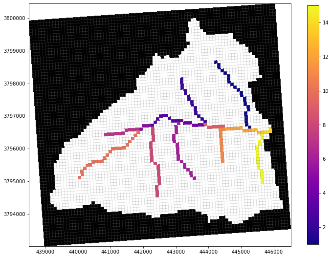
Let’s plot the stream network from SFR first, just to examine it.
[4]:
rch = gsf.mf.sfr.reach_data

# set up an array of iseg numbers to visualize connectivity
arr = np.zeros((1, gsf.mf.nrow, gsf.mf.ncol), dtype='int')
for rec in rch:
    arr[0, rec.i, rec.j] = rec.iseg

# use flopy to plot the SFR segments
fig = plt.figure(figsize=(12, 12))
pmv = fp.plot.PlotMapView(model=gsf.mf)
collection = pmv.plot_array(arr, masked_values=[0,], cmap='plasma')
pmv.plot_inactive()
pmv.plot_grid(lw=0.25)
plt.colorbar(collection, shrink=0.75);
Creating a Modsim instance using a GsflowModel object
creating a MODSIM instance is as easy as passing a GsflowModel object to the Modsim class.
[5]:
# creating a MODSIM instance is as easy as
modsim = gsflow.modsim.Modsim(gsf)
Exporting a vector shapefile from Modsim
The Modsim instance has a built in method write_modsim_shapefile() that is used to write a stream vector shapefiles. The write_modsim_shapefile has a number of parameters that can be used:
shp: is a string defining the output shapefile’s nameproj4: proj4 is an optional parameter that can be used to define the shapefile’s projection informationflag_spillway: an optional parameter that can be used to determine spillways in the streamflow network. There are methods that have been implemented +"elev": elevation method which flags based on streambed elevation rules +"flow": flag spillways based on flow rules + list of segments : the user can provide a list of segments that are known spillways to be flaggednearest: boolean value that determines if LAK topology will connect to the nearest reach in a segment or the the begining/end of that segment.
[6]:
shp_file = os.path.join(ws, "data", "temp", "sagehen_vectors.shp")
modsim.write_modsim_shapefile(shp_file)
modsim.py:361: UserWarning: Please provide a valid proj4 or epsg code to flopy'smodel grid: Skipping writing sagehen_vectors.prj
Checking the attribute table
Now that the shapefile has been created it can be loaded into GIS software and analyzed. Note: In this example I did not define a projection, and would then need to assign it using my GIS software’s tools.
We can also use pyshp to load the shapefile and inspect it in python.
[7]:
attr = []
shps = {}
with shapefile.Reader(shp_file) as r:
    fields = [f[0] for i, f in enumerate(r.fields) if i > 0]
    for ix, shape in enumerate(r.shapes()):
        feat = shape.__geo_interface__
        xy = np.array(feat['coordinates']).T
        shps[ix] = xy
        rec = [i for i in r.record(ix)]
        attr.append(rec)

df = pd.DataFrame(attr, columns=fields)
df
[7]:
| ISEG | IUPSEG | OUTSEG | SPILL_FLG | |
|---|---|---|---|---|
| 0 | 1 | 0 | 13 | 0 |
| 1 | 2 | 0 | 9 | 0 |
| 2 | 3 | 0 | 4 | 0 |
| 3 | 4 | 0 | 9 | 0 |
| 4 | 5 | 0 | 3 | 0 |
| 5 | 6 | 0 | 4 | 0 |
| 6 | 7 | 0 | 5 | 0 |
| 7 | 8 | 0 | 3 | 0 |
| 8 | 9 | 0 | 12 | 0 |
| 9 | 10 | 0 | 5 | 0 |
| 10 | 11 | 0 | 12 | 0 |
| 11 | 12 | 0 | 13 | 0 |
| 12 | 13 | 0 | 14 | 0 |
| 13 | 14 | 0 | 0 | 0 |
| 14 | 15 | 0 | 14 | 0 |
[8]:
# use flopy to plot the SFR segments
fig = plt.figure(figsize=(10, 10))
pmv = fp.plot.PlotMapView(model=gsf.mf)
# collection = pmv.plot_array(arr, masked_values=[0,], cmap='plasma')
pmv.plot_inactive()
pmv.plot_grid(lw=0.25)
pmv.plot_bc(package=gsf.mf.sfr, color='gainsboro')
for _, xy in shps.items():
    plt.plot(xy[0], xy[1], lw=2)

plt.title("Stream vector plot");

Modflow instances can also be used to create a vector shapefile
The Modsim class can also accept a flopy.modflow.Modflow object to create a vector shapefile
[9]:
ml = fp.modflow.Modflow.load('saghen_new.nam', model_ws=model_ws, version='mfnwt')
ml.modelgrid.set_coord_info(xll, yll, angrot)

modsim = gsflow.modsim.Modsim(ml)

shp_file = os.path.join(ws, "data", "temp", "sagehen_modflow_vectors.shp")
modsim.write_modsim_shapefile(shp_file)
   loading iuzfbnd array...
   loading irunbnd array...
   loading vks array...
   loading eps array...
   loading thts array...
stress period 1:
   loading finf array...
stress period 2:
Inspecting the shapefile:
[10]:
attr = []
shps = {}
with shapefile.Reader(shp_file) as r:
    fields = [f[0] for i, f in enumerate(r.fields) if i > 0]
    for ix, shape in enumerate(r.shapes()):
        feat = shape.__geo_interface__
        xy = np.array(feat['coordinates']).T
        shps[ix] = xy
        rec = [i for i in r.record(ix)]
        attr.append(rec)

df = pd.DataFrame(attr, columns=fields)
df
[10]:
| ISEG | IUPSEG | OUTSEG | SPILL_FLG | |
|---|---|---|---|---|
| 0 | 1 | 0 | 13 | 0 |
| 1 | 2 | 0 | 9 | 0 |
| 2 | 3 | 0 | 4 | 0 |
| 3 | 4 | 0 | 9 | 0 |
| 4 | 5 | 0 | 3 | 0 |
| 5 | 6 | 0 | 4 | 0 |
| 6 | 7 | 0 | 5 | 0 |
| 7 | 8 | 0 | 3 | 0 |
| 8 | 9 | 0 | 12 | 0 |
| 9 | 10 | 0 | 5 | 0 |
| 10 | 11 | 0 | 12 | 0 |
| 11 | 12 | 0 | 13 | 0 |
| 12 | 13 | 0 | 14 | 0 |
| 13 | 14 | 0 | 0 | 0 |
| 14 | 15 | 0 | 14 | 0 |
[11]:
# use flopy to plot the SFR segments
fig = plt.figure(figsize=(10, 10))
pmv = fp.plot.PlotMapView(model=ml)
# collection = pmv.plot_array(arr, masked_values=[0,], cmap='plasma')
pmv.plot_inactive()
pmv.plot_grid(lw=0.25)
pmv.plot_bc(package=ml.sfr, color='gainsboro')
for _, xy in shps.items():
    plt.plot(xy[0], xy[1], lw=2)

plt.title("Stream vector plot");
[ ]: